User Guide¶

SPFlow is an open-source functional-oriented Python package for Probabilistic Circuits (PCs) with ready-to-use implementations for Sum-Product Networks (SPNs). PCs are a class of powerful deep probabilistic models - expressible as directed acyclic graphs - that allow for tractable querying. This library provides routines for creating, learning, manipulating and interacting with PCs and is highly extensible and customizable.

Create Toy Dataset¶

To demonstrate and visualize the main features of the library, we first create a 2D toy dataset with three Gaussian clusters, corresponding to labels 0, 1, and 2. The dataset is created with an imbalance. Therefore, class 0 has 200 datapoints, class 1 400 datapoints and class 2 600 datapoints, for a total of 1,200 data points.

[26]:

import torch
import matplotlib.pyplot as plt
import numpy as np

# --- 1. Define the parameters for our dataset ---

n_points_per_cluster = 200

means = torch.tensor([
    [0.0, 3.0],  # Cluster 0
    [-3.0, -2.0],  # Cluster 1
    [3.0, -2.0]  # Cluster 2
])

stds = torch.tensor([
    [0.6, 0.6],
    [0.8, 0.4],
    [0.5, 0.7]
])

# --- 2. Generate the data and labels ---

all_clusters = []
all_labels = []

for i in range(means.shape[0]):
    samples = (torch.randn(n_points_per_cluster * (i + 1), 2) * stds[i]) + means[i]
    labels = torch.full((n_points_per_cluster * (i + 1),), i, dtype=torch.long)  # label = cluster index
    all_clusters.append(samples)
    all_labels.append(labels)

# Concatenate all data and labels
dataset = torch.cat(all_clusters)
labels = torch.cat(all_labels)

# --- 3. Shuffle dataset and labels together ---

shuffled_indices = torch.randperm(dataset.shape[0])
dataset = dataset[shuffled_indices]
labels = labels[shuffled_indices]

# --- 4. Display some info ---

print("Dataset successfully created.")
print(f"Shape of dataset: {dataset.shape}")
print(f"Shape of labels: {labels.shape}")
print("First 5 samples:")
print(dataset[:5])
print("Corresponding labels:")
print(labels[:5])

# --- 5. Visualize the labeled dataset ---

data_np = dataset.cpu().numpy()
labels_np = labels.cpu().numpy()


def plot_scatter(data_list, title=None, labels=None, label_list=None):
    colors = ["blue", "red", "yellow", "green"]
    plt.figure(figsize=(8, 6))
    for idx, data in enumerate(data_list):
        print(len(data_list))
        print(data.shape)
        print(label_list[idx])
        if labels is not None and len(data_list) == 1:
            plt.scatter(data[:, 0], data[:, 1], c=labels, cmap="viridis", s=10, alpha=0.7)
            plt.colorbar(label='Cluster Label')
        else:
            plt.scatter(data[:, 0], data[:, 1], c=colors[idx], s=10, alpha=0.7, label=label_list[idx])
            plt.legend()

    plt.title(title)
    plt.xlabel('Feature 1 (x-axis)')
    plt.ylabel('Feature 2 (y-axis)')
    plt.grid(True, linestyle='--', alpha=0.6)
    plt.axis('equal')
    #plt.colorbar(label='Cluster Label')

    plt.show()


plot_scatter([data_np], title='Generated 2D Toy Dataset (with Labels)', labels=labels_np, label_list=['Toy Data'])

Dataset successfully created.
Shape of dataset: torch.Size([1200, 2])
Shape of labels: torch.Size([1200])
First 5 samples:
tensor([[-3.4324, -2.0308],
        [-2.7769, -2.2276],
        [ 2.8235, -3.4650],
        [ 2.9876, -1.5170],
        [ 0.3865,  3.5942]])
Corresponding labels:
tensor([1, 1, 2, 2, 0])
1
(1200, 2)
Toy Data

Model Configuration¶

The circuits you create with this library are modular.

All modules share the same base structure. Each module is defined by its number of output features and output channels. You can think of output features as the number of nodes with different scopes in one layer. You can think of output channels as how many times a node with the same scope is repeated in a layer. This structure lets you define simple nodes (with a shape of (1, 1)), node vectors along the feature (N, 1) or channel (1, M) dimension, or full leaf layers (N, M). In many cases, using layers instead of single nodes is much faster and more memory-efficient.

Each module also has an input attribute that points to its input module. This lets you stack modules together in any order.

Below, we will build a simple Sum-Product Network by stacking leaf, product, and sum layers.

[27]:

from spflow.modules.leaves import Normal
from spflow.modules.sums import Sum
from spflow.modules.products import Product
from spflow.meta.data import Scope
from IPython.display import display, Image

scope = Scope([0, 1])

leaf_layer = Normal(scope=scope, out_channels=6)
product_layer = Product(inputs=leaf_layer)
spn = Sum(inputs=product_layer, out_channels=1)
spn

[27]:

Sum(
  D=1, C=1, R=1, weights=(1, 6, 1, 1)
  (inputs): Product(
    D=1, C=6, R=1
    (inputs): Normal(D=2, C=6, R=1)
  )
)

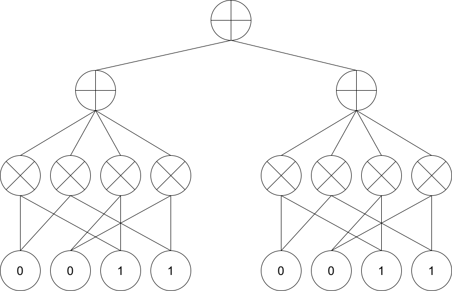
Below is a visualization of the SPN defined above. The number of output channels of a sum or leaf layer is equivalent to the number of nodes in that layer. The number of nodes in a product layer is derived from the number of nodes in its input.

[28]:

display(Image(filename='StandardSPN.png'))

Next, we can train the SPN, for example, using gradient descent. The library already provides a method for training an SPN with gradient descent. To do this, simply pass the module you want to train and the training parameters such as the number of epochs, learning rate, etc.

[29]:

from spflow.learn import train_gradient_descent
from torch.utils.data import DataLoader, TensorDataset
import logging

logging.basicConfig(
    level=logging.INFO,
    format="%(asctime)s [%(levelname)s] %(name)s: %(message)s"
)

train_dataset = TensorDataset(dataset)
dataloader = DataLoader(train_dataset, batch_size=10)
train_gradient_descent(spn, dataloader, epochs=10, lr=0.1, verbose=True)

2025-12-30 11:50:30,025 [INFO] spflow.learn.gradient_descent: Epoch [0/10]: Loss: 3.2784781455993652
2025-12-30 11:50:30,047 [INFO] spflow.learn.gradient_descent: Epoch [1/10]: Loss: 3.1120753288269043
2025-12-30 11:50:30,069 [INFO] spflow.learn.gradient_descent: Epoch [2/10]: Loss: 3.089931011199951
2025-12-30 11:50:30,089 [INFO] spflow.learn.gradient_descent: Epoch [3/10]: Loss: 3.0767736434936523
2025-12-30 11:50:30,110 [INFO] spflow.learn.gradient_descent: Epoch [4/10]: Loss: 3.068474531173706
2025-12-30 11:50:30,130 [INFO] spflow.learn.gradient_descent: Epoch [5/10]: Loss: 2.927799701690674
2025-12-30 11:50:30,151 [INFO] spflow.learn.gradient_descent: Epoch [6/10]: Loss: 2.923741579055786
2025-12-30 11:50:30,172 [INFO] spflow.learn.gradient_descent: Epoch [7/10]: Loss: 2.912303924560547
2025-12-30 11:50:30,193 [INFO] spflow.learn.gradient_descent: Epoch [8/10]: Loss: 2.9066848754882812
2025-12-30 11:50:30,214 [INFO] spflow.learn.gradient_descent: Epoch [9/10]: Loss: 2.9028568267822266

Once the SPN is trained, we can perform queries such as inference and sampling. SPFlow uses internal dispatching so that a single query function can work across all module types. For example, the log_likelihood method shown below can be used for every SPN model encountered throughout this guide.

[30]:

ll = spn.log_likelihood(dataset)
ll

[30]:

tensor([[[[-1.9579]]],


        [[[-2.1401]]],


        [[[-3.6376]]],


        ...,


        [[[-5.6696]]],


        [[[-2.4165]]],


        [[[-1.6529]]]], grad_fn=<ViewBackward0>)

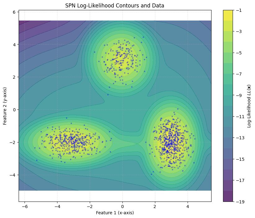
Finally, we can visualize the training results on our toy dataset.

[31]:

data_np = dataset.cpu().numpy()


def plot_contour(data, spn):
    # Define the boundaries of the plot with a small padding
    x_min, x_max = data_np[:, 0].min() - 1, data_np[:, 0].max() + 1
    y_min, y_max = data_np[:, 1].min() - 1, data_np[:, 1].max() + 1

    # Create a grid of points
    grid_resolution = 200
    xx, yy = np.meshgrid(np.linspace(x_min, x_max, grid_resolution),
                         np.linspace(y_min, y_max, grid_resolution))

    # Stack the grid points into a format our function can accept: [n_points, 2]
    grid_points = torch.tensor(np.c_[xx.ravel(), yy.ravel()], dtype=torch.float32)
    ll = spn.log_likelihood(grid_points)
    # Reshape the LL values to match the grid shape for plotting
    Z = ll.detach().cpu().numpy().reshape(xx.shape)

    # --- 6. Visualize the Data and Log-Likelihood Contours ---

    plt.figure(figsize=(10, 8))

    # Plot the filled contour map of the log-likelihood
    # Higher values (brighter colors) mean the model thinks data is more likely there
    contour = plt.contourf(xx, yy, Z, levels=20, cmap='viridis', alpha=0.8)

    # Add a color bar to show the LL scale
    plt.colorbar(contour, label='Log-Likelihood $LL(\mathbf{x})$')

    # Overlay the scatter plot of the actual data points
    # We make them semi-transparent and small to see the density and contours
    plt.scatter(data_np[:, 0], data_np[:, 1], s=5, alpha=0.3, c='blue')

    # Add titles and labels
    plt.title('SPN Log-Likelihood Contours and Data')
    plt.xlabel('Feature 1 (x-axis)')
    plt.ylabel('Feature 2 (y-axis)')
    plt.grid(True, linestyle='--', alpha=0.3)
    plt.axis('equal')  # Ensures the scaling is the same on both axes
    plt.show()


plot_contour(data_np, spn)

<>:29: SyntaxWarning: invalid escape sequence '\m'
<>:29: SyntaxWarning: invalid escape sequence '\m'
/var/folders/t3/57fhyt955l9d7dby5dmlzs900000gn/T/ipykernel_94580/3280425296.py:29: SyntaxWarning: invalid escape sequence '\m'
  plt.colorbar(contour, label='Log-Likelihood $LL(\mathbf{x})$')

Temporary Method Replacement¶

SPFlow supports temporarily substituting module methods. For example, you can replace the sum operation in Sum with a custom implementation for a single call graph.

[32]:

import torch
from spflow.modules.sums import Sum
from spflow.modules.products import Product
from spflow.modules.leaves import Normal
from spflow.meta import Scope
from spflow.utils import replace

torch.manual_seed(1)

# Create a probabilistic circuit: Product(Sum(Product(Normal)))
scope = Scope([0, 1])
normal = Normal(scope=scope, out_channels=4)
inner_product = Product(inputs=normal)
sum_module = Sum(inputs=inner_product, out_channels=1)
root_product = Product(inputs=sum_module)

# Create test data
data = torch.randn(3, 2)

# Normal inference
log_likelihood_original = root_product.log_likelihood(data).flatten()
print(f"Original log-likelihood: {log_likelihood_original}")

# Define a custom log_likelihood for Sum modules
def max_ll(self, data, cache=None):
    ll = self.inputs.log_likelihood(data, cache=cache).unsqueeze(3)
    weighted_lls = ll + self.log_weights.unsqueeze(0)
    return torch.max(weighted_lls, dim=self.sum_dim + 1)[0]

# Temporarily replace Sum.log_likelihood with custom implementation
with replace(Sum.log_likelihood, max_ll):
    log_likelihood_custom = root_product.log_likelihood(data).flatten()
    print(f"Custom log-likelihood:   {log_likelihood_custom}")

# Original method is automatically restored
log_likelihood_restored = root_product.log_likelihood(data).flatten()
print(f"Restored log-likelihood: {log_likelihood_restored}")

Original log-likelihood: tensor([-1.2842, -2.8750, -7.2442], grad_fn=<ViewBackward0>)
Custom log-likelihood:   tensor([-1.4334, -3.5256, -7.9031], grad_fn=<ViewBackward0>)
Restored log-likelihood: tensor([-1.2842, -2.8750, -7.2442], grad_fn=<ViewBackward0>)

Automatic Model creation¶

Besides creating an SPN manually by stacking layers, it is also possible to use algorithms to automatically construct the SPN architecture. This can make it easier to start using SPNs.

Rat-SPN¶

The Rat-SPN algorithm builds a deep network structure by recursively partitioning the features (variables) into random subsets and alternating between sum and product layers. Below, we set up a Rat-SPN by defining its structure and parameters.

[33]:

from spflow.modules.rat.rat_spn import RatSPN
from spflow.modules.ops.split import SplitMode

depth = 1
n_region_nodes = 3
num_leaves = 2
num_repetitions = 2
n_root_nodes = 1
num_feature = 2

scope = Scope(list(range(0, num_feature)))

rat_leaf_layer = Normal(scope=scope, out_channels=num_leaves, num_repetitions=num_repetitions)
rat = RatSPN(
    leaf_modules=[rat_leaf_layer],
    n_root_nodes=n_root_nodes,
    n_region_nodes=n_region_nodes,
    num_repetitions=num_repetitions,
    depth=depth,
    outer_product=True,
    split_mode=SplitMode.consecutive(),
)
print(rat.to_str())

RatSPN [D=1, C=1, R=2] → scope: 0-1
└─ RepetitionMixingLayer [D=1, C=1] [weights: (1, 1, 2)] → scope: 0-1
   └─ Sum [D=1, C=1] [weights: (1, 4, 1, 2)] → scope: 0-1
      └─ OuterProduct [D=1, C=4] → scope: 0-1
         └─ SplitConsecutive [D=2, C=2] → scope: 0-1
            └─ Factorize [D=2, C=2] → scope: 0-1
               └─ Normal [D=2, C=2] → scope: 0-1

Here is a visualization of the architecture we just created.

[34]:

display(Image(filename='Rat_SPN.png'))

[35]:

ll = rat.log_likelihood(dataset)
ll

[35]:

tensor([[[[-11.5142]]],


        [[[ -9.2007]]],


        [[[-21.5388]]],


        ...,


        [[[ -4.4811]]],


        [[[ -8.0701]]],


        [[[-11.3642]]]], grad_fn=<ViewBackward0>)

We can again train this model using the provided gradient descent method.

[36]:

train_gradient_descent(rat, dataloader, epochs=20, lr=0.1)

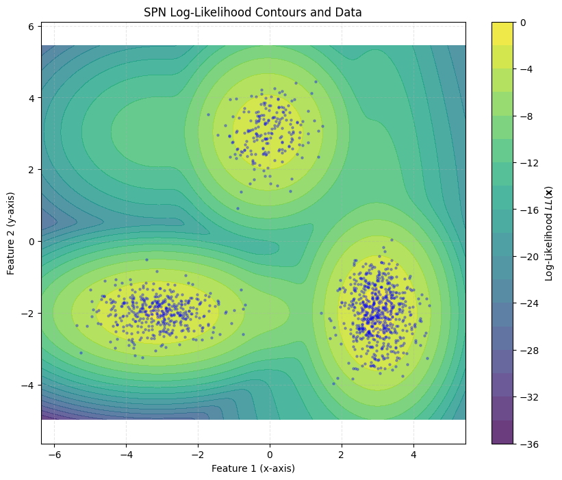
To verify that the training worked properly, we can visualize the log-likelihoods of the trained model.

[37]:

data_np = dataset.cpu().numpy()
plot_contour(data_np, rat)

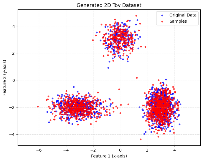
Of course, computing log-likelihoods is not the only thing the model can do. Below is a visualization of samples drawn from the trained Rat-SPN.

[38]:

samples = spn.sample(num_samples=1500)
plot_scatter([data_np, samples], title='Generated 2D Toy Dataset', label_list=['Original Data', 'Samples'])

2
(1200, 2)
Original Data
2
torch.Size([1500, 2])
Samples

Up to now, we have focused only on generation, without considering the labels of the training instances. Next, we will train a second Rat-SPN for classification.

[39]:

import logging

logging.basicConfig(
    level=logging.INFO,
    format="%(asctime)s [%(levelname)s] %(name)s: %(message)s"
)

depth = 1
n_region_nodes = 3
num_leaves = 3
num_repetitions = 1
n_root_nodes = 3
num_feature = 2

scope = Scope(list(range(0, num_feature)))

rat_leaf_layer = Normal(scope=scope, out_channels=num_leaves, num_repetitions=num_repetitions)
rat_class = RatSPN(
    leaf_modules=[rat_leaf_layer],
    n_root_nodes=n_root_nodes,
    n_region_nodes=n_region_nodes,
    num_repetitions=num_repetitions,
    depth=depth,
    outer_product=True,
    split_mode=SplitMode.consecutive(),
)
train_dataset = TensorDataset(dataset.clone(), labels.clone())

dataloader_with_labels = DataLoader(train_dataset, batch_size=10)

train_gradient_descent(rat_class, dataloader_with_labels, epochs=100, lr=0.1, is_classification=True,
                       verbose=True)

2025-12-30 11:50:31,271 [INFO] spflow.learn.gradient_descent: Epoch [0/100]: Loss: 2.065856456756592
2025-12-30 11:50:31,373 [INFO] spflow.learn.gradient_descent: Epoch [1/100]: Loss: 2.0176610946655273
2025-12-30 11:50:31,475 [INFO] spflow.learn.gradient_descent: Epoch [2/100]: Loss: 2.0115408897399902
2025-12-30 11:50:31,574 [INFO] spflow.learn.gradient_descent: Epoch [3/100]: Loss: 2.007749557495117
2025-12-30 11:50:31,668 [INFO] spflow.learn.gradient_descent: Epoch [4/100]: Loss: 2.005401611328125
2025-12-30 11:50:31,763 [INFO] spflow.learn.gradient_descent: Epoch [5/100]: Loss: 2.0036461353302
2025-12-30 11:50:31,858 [INFO] spflow.learn.gradient_descent: Epoch [6/100]: Loss: 2.002192258834839
2025-12-30 11:50:31,951 [INFO] spflow.learn.gradient_descent: Epoch [7/100]: Loss: 2.0010249614715576
2025-12-30 11:50:32,044 [INFO] spflow.learn.gradient_descent: Epoch [8/100]: Loss: 2.0139596462249756
2025-12-30 11:50:32,136 [INFO] spflow.learn.gradient_descent: Epoch [9/100]: Loss: 2.002393960952759
2025-12-30 11:50:32,228 [INFO] spflow.learn.gradient_descent: Epoch [10/100]: Loss: 1.9963277578353882
2025-12-30 11:50:32,320 [INFO] spflow.learn.gradient_descent: Epoch [11/100]: Loss: 1.999521017074585
2025-12-30 11:50:32,414 [INFO] spflow.learn.gradient_descent: Epoch [12/100]: Loss: 1.9988003969192505
2025-12-30 11:50:32,506 [INFO] spflow.learn.gradient_descent: Epoch [13/100]: Loss: 1.9983843564987183
2025-12-30 11:50:32,597 [INFO] spflow.learn.gradient_descent: Epoch [14/100]: Loss: 1.9982181787490845
2025-12-30 11:50:32,688 [INFO] spflow.learn.gradient_descent: Epoch [15/100]: Loss: 1.9981024265289307
2025-12-30 11:50:32,779 [INFO] spflow.learn.gradient_descent: Epoch [16/100]: Loss: 1.9979139566421509
2025-12-30 11:50:32,872 [INFO] spflow.learn.gradient_descent: Epoch [17/100]: Loss: 2.0082948207855225
2025-12-30 11:50:32,963 [INFO] spflow.learn.gradient_descent: Epoch [18/100]: Loss: 1.999101161956787
2025-12-30 11:50:33,055 [INFO] spflow.learn.gradient_descent: Epoch [19/100]: Loss: 1.9988633394241333
2025-12-30 11:50:33,146 [INFO] spflow.learn.gradient_descent: Epoch [20/100]: Loss: 1.9988266229629517
2025-12-30 11:50:33,237 [INFO] spflow.learn.gradient_descent: Epoch [21/100]: Loss: 1.9967951774597168
2025-12-30 11:50:33,327 [INFO] spflow.learn.gradient_descent: Epoch [22/100]: Loss: 2.000103235244751
2025-12-30 11:50:33,421 [INFO] spflow.learn.gradient_descent: Epoch [23/100]: Loss: 2.000051498413086
2025-12-30 11:50:33,511 [INFO] spflow.learn.gradient_descent: Epoch [24/100]: Loss: 2.0000452995300293
2025-12-30 11:50:33,602 [INFO] spflow.learn.gradient_descent: Epoch [25/100]: Loss: 2.000060558319092
2025-12-30 11:50:33,693 [INFO] spflow.learn.gradient_descent: Epoch [26/100]: Loss: 2.0000829696655273
2025-12-30 11:50:33,790 [INFO] spflow.learn.gradient_descent: Epoch [27/100]: Loss: 2.000107526779175
2025-12-30 11:50:33,893 [INFO] spflow.learn.gradient_descent: Epoch [28/100]: Loss: 2.0001320838928223
2025-12-30 11:50:33,992 [INFO] spflow.learn.gradient_descent: Epoch [29/100]: Loss: 2.000155448913574
2025-12-30 11:50:34,089 [INFO] spflow.learn.gradient_descent: Epoch [30/100]: Loss: 2.0001778602600098
2025-12-30 11:50:34,186 [INFO] spflow.learn.gradient_descent: Epoch [31/100]: Loss: 2.0001978874206543
2025-12-30 11:50:34,281 [INFO] spflow.learn.gradient_descent: Epoch [32/100]: Loss: 2.000215768814087
2025-12-30 11:50:34,374 [INFO] spflow.learn.gradient_descent: Epoch [33/100]: Loss: 2.000232458114624
2025-12-30 11:50:34,467 [INFO] spflow.learn.gradient_descent: Epoch [34/100]: Loss: 2.000246524810791
2025-12-30 11:50:34,559 [INFO] spflow.learn.gradient_descent: Epoch [35/100]: Loss: 2.0002593994140625
2025-12-30 11:50:34,653 [INFO] spflow.learn.gradient_descent: Epoch [36/100]: Loss: 2.000270366668701
2025-12-30 11:50:34,748 [INFO] spflow.learn.gradient_descent: Epoch [37/100]: Loss: 2.0002799034118652
2025-12-30 11:50:34,845 [INFO] spflow.learn.gradient_descent: Epoch [38/100]: Loss: 2.000288486480713
2025-12-30 11:50:34,941 [INFO] spflow.learn.gradient_descent: Epoch [39/100]: Loss: 2.000296115875244
2025-12-30 11:50:35,034 [INFO] spflow.learn.gradient_descent: Epoch [40/100]: Loss: 2.000302314758301
2025-12-30 11:50:35,125 [INFO] spflow.learn.gradient_descent: Epoch [41/100]: Loss: 2.000307559967041
2025-12-30 11:50:35,216 [INFO] spflow.learn.gradient_descent: Epoch [42/100]: Loss: 2.000312328338623
2025-12-30 11:50:35,306 [INFO] spflow.learn.gradient_descent: Epoch [43/100]: Loss: 2.000316619873047
2025-12-30 11:50:35,397 [INFO] spflow.learn.gradient_descent: Epoch [44/100]: Loss: 2.000319719314575
2025-12-30 11:50:35,488 [INFO] spflow.learn.gradient_descent: Epoch [45/100]: Loss: 2.0003223419189453
2025-12-30 11:50:35,578 [INFO] spflow.learn.gradient_descent: Epoch [46/100]: Loss: 2.0003247261047363
2025-12-30 11:50:35,669 [INFO] spflow.learn.gradient_descent: Epoch [47/100]: Loss: 2.000326633453369
2025-12-30 11:50:35,759 [INFO] spflow.learn.gradient_descent: Epoch [48/100]: Loss: 2.000328302383423
2025-12-30 11:50:35,849 [INFO] spflow.learn.gradient_descent: Epoch [49/100]: Loss: 2.0003292560577393
2025-12-30 11:50:35,945 [INFO] spflow.learn.gradient_descent: Epoch [50/100]: Loss: 1.8605408668518066
2025-12-30 11:50:36,038 [INFO] spflow.learn.gradient_descent: Epoch [51/100]: Loss: 1.8524022102355957
2025-12-30 11:50:36,129 [INFO] spflow.learn.gradient_descent: Epoch [52/100]: Loss: 1.8517446517944336
2025-12-30 11:50:36,220 [INFO] spflow.learn.gradient_descent: Epoch [53/100]: Loss: 1.8516888618469238
2025-12-30 11:50:36,310 [INFO] spflow.learn.gradient_descent: Epoch [54/100]: Loss: 1.8516950607299805
2025-12-30 11:50:36,403 [INFO] spflow.learn.gradient_descent: Epoch [55/100]: Loss: 1.8517076969146729
2025-12-30 11:50:36,496 [INFO] spflow.learn.gradient_descent: Epoch [56/100]: Loss: 1.8517193794250488
2025-12-30 11:50:36,586 [INFO] spflow.learn.gradient_descent: Epoch [57/100]: Loss: 1.8517301082611084
2025-12-30 11:50:36,678 [INFO] spflow.learn.gradient_descent: Epoch [58/100]: Loss: 1.8517398834228516
2025-12-30 11:50:36,768 [INFO] spflow.learn.gradient_descent: Epoch [59/100]: Loss: 1.8517487049102783
2025-12-30 11:50:36,862 [INFO] spflow.learn.gradient_descent: Epoch [60/100]: Loss: 1.8517558574676514
2025-12-30 11:50:36,955 [INFO] spflow.learn.gradient_descent: Epoch [61/100]: Loss: 1.8517637252807617
2025-12-30 11:50:37,045 [INFO] spflow.learn.gradient_descent: Epoch [62/100]: Loss: 1.8517695665359497
2025-12-30 11:50:37,136 [INFO] spflow.learn.gradient_descent: Epoch [63/100]: Loss: 1.8517755270004272
2025-12-30 11:50:37,226 [INFO] spflow.learn.gradient_descent: Epoch [64/100]: Loss: 1.851779818534851
2025-12-30 11:50:37,316 [INFO] spflow.learn.gradient_descent: Epoch [65/100]: Loss: 1.851784586906433
2025-12-30 11:50:37,408 [INFO] spflow.learn.gradient_descent: Epoch [66/100]: Loss: 1.8517884016036987
2025-12-30 11:50:37,506 [INFO] spflow.learn.gradient_descent: Epoch [67/100]: Loss: 1.8517922163009644
2025-12-30 11:50:37,599 [INFO] spflow.learn.gradient_descent: Epoch [68/100]: Loss: 1.851794719696045
2025-12-30 11:50:37,691 [INFO] spflow.learn.gradient_descent: Epoch [69/100]: Loss: 1.8517974615097046
2025-12-30 11:50:37,782 [INFO] spflow.learn.gradient_descent: Epoch [70/100]: Loss: 1.8517998456954956
2025-12-30 11:50:37,872 [INFO] spflow.learn.gradient_descent: Epoch [71/100]: Loss: 1.8518023490905762
2025-12-30 11:50:37,965 [INFO] spflow.learn.gradient_descent: Epoch [72/100]: Loss: 1.851803183555603
2025-12-30 11:50:38,056 [INFO] spflow.learn.gradient_descent: Epoch [73/100]: Loss: 1.8518047332763672
2025-12-30 11:50:38,146 [INFO] spflow.learn.gradient_descent: Epoch [74/100]: Loss: 1.8518059253692627
2025-12-30 11:50:38,237 [INFO] spflow.learn.gradient_descent: Epoch [75/100]: Loss: 1.8459644317626953
2025-12-30 11:50:38,327 [INFO] spflow.learn.gradient_descent: Epoch [76/100]: Loss: 1.8435673713684082
2025-12-30 11:50:38,419 [INFO] spflow.learn.gradient_descent: Epoch [77/100]: Loss: 1.842025876045227
2025-12-30 11:50:38,511 [INFO] spflow.learn.gradient_descent: Epoch [78/100]: Loss: 1.8409959077835083
2025-12-30 11:50:38,602 [INFO] spflow.learn.gradient_descent: Epoch [79/100]: Loss: 1.8402832746505737
2025-12-30 11:50:38,693 [INFO] spflow.learn.gradient_descent: Epoch [80/100]: Loss: 1.8397735357284546
2025-12-30 11:50:38,783 [INFO] spflow.learn.gradient_descent: Epoch [81/100]: Loss: 1.8393982648849487
2025-12-30 11:50:38,873 [INFO] spflow.learn.gradient_descent: Epoch [82/100]: Loss: 1.8391164541244507
2025-12-30 11:50:38,966 [INFO] spflow.learn.gradient_descent: Epoch [83/100]: Loss: 1.8389016389846802
2025-12-30 11:50:39,062 [INFO] spflow.learn.gradient_descent: Epoch [84/100]: Loss: 1.8387354612350464
2025-12-30 11:50:39,154 [INFO] spflow.learn.gradient_descent: Epoch [85/100]: Loss: 1.8386057615280151
2025-12-30 11:50:39,245 [INFO] spflow.learn.gradient_descent: Epoch [86/100]: Loss: 1.8385034799575806
2025-12-30 11:50:39,336 [INFO] spflow.learn.gradient_descent: Epoch [87/100]: Loss: 1.8384226560592651
2025-12-30 11:50:39,430 [INFO] spflow.learn.gradient_descent: Epoch [88/100]: Loss: 1.838358759880066
2025-12-30 11:50:39,523 [INFO] spflow.learn.gradient_descent: Epoch [89/100]: Loss: 1.8383077383041382
2025-12-30 11:50:39,614 [INFO] spflow.learn.gradient_descent: Epoch [90/100]: Loss: 1.8382673263549805
2025-12-30 11:50:39,707 [INFO] spflow.learn.gradient_descent: Epoch [91/100]: Loss: 1.8382349014282227
2025-12-30 11:50:39,798 [INFO] spflow.learn.gradient_descent: Epoch [92/100]: Loss: 1.8382089138031006
2025-12-30 11:50:39,890 [INFO] spflow.learn.gradient_descent: Epoch [93/100]: Loss: 1.838188886642456
2025-12-30 11:50:39,986 [INFO] spflow.learn.gradient_descent: Epoch [94/100]: Loss: 1.8381726741790771
2025-12-30 11:50:40,077 [INFO] spflow.learn.gradient_descent: Epoch [95/100]: Loss: 1.8381595611572266
2025-12-30 11:50:40,169 [INFO] spflow.learn.gradient_descent: Epoch [96/100]: Loss: 1.8381495475769043
2025-12-30 11:50:40,259 [INFO] spflow.learn.gradient_descent: Epoch [97/100]: Loss: 1.8381412029266357
2025-12-30 11:50:40,349 [INFO] spflow.learn.gradient_descent: Epoch [98/100]: Loss: 1.838134527206421
2025-12-30 11:50:40,440 [INFO] spflow.learn.gradient_descent: Epoch [99/100]: Loss: 1.8381297588348389

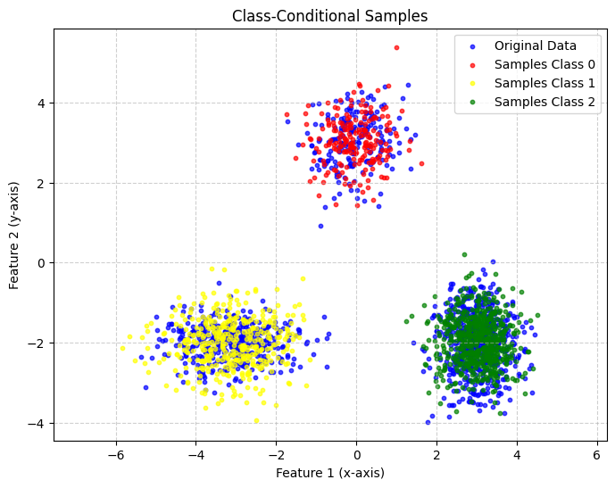
With this SPN, we can now draw samples based on its labels. Therefore, we use a sampling context. This sampling context can be passed to any sampling method. With the context, you can explicitly define from which output channel you want to sample or, for example, provide evidence. This allows advanced control over the sampling routine. In this case, the root layer has three output channels which correspond to the three classes. So being able to define from which output channel we want to sample means being able to choose from which class we want to sample.

[40]:

from spflow.utils.sampling_context import SamplingContext

out_features = rat.out_shape.features
num_features = 2

evidence = torch.full((200, num_features), torch.nan)
channel_index = torch.full((200, out_features), 0, dtype=torch.int64)
mask = torch.full((200, out_features), True, dtype=torch.bool)
sampling_ctx = SamplingContext(channel_index=channel_index, mask=mask)
samples_class0 = rat_class.root_node.inputs.sample(data=evidence, sampling_ctx=sampling_ctx)

evidence = torch.full((400, num_features), torch.nan)
channel_index = torch.full((400, out_features), 1, dtype=torch.int64)
mask = torch.full((400, out_features), True, dtype=torch.bool)
sampling_ctx = SamplingContext(channel_index=channel_index, mask=mask)
samples_class1 = rat_class.sample(data=evidence, sampling_ctx=sampling_ctx)

evidence = torch.full((600, num_features), torch.nan)
channel_index = torch.full((600, out_features), 2, dtype=torch.int64)
mask = torch.full((600, out_features), True, dtype=torch.bool)
sampling_ctx = SamplingContext(channel_index=channel_index, mask=mask)
samples_class2 = rat_class.sample(data=evidence, sampling_ctx=sampling_ctx)

plot_scatter([data_np, samples_class0, samples_class1, samples_class2], title='Class-Conditional Samples',
             label_list=['Original Data', 'Samples Class 0', 'Samples Class 1', 'Samples Class 2'])

4
(1200, 2)
Original Data
4
torch.Size([200, 2])
Samples Class 0
4
torch.Size([400, 2])
Samples Class 1
4
torch.Size([600, 2])
Samples Class 2

However, the model can of course also be used for classification. As an example, we visualize the trained decision boundaries of our model

[41]:

import torch
import matplotlib.pyplot as plt
import numpy as np

# --- Assuming your dataset and labels are already created as above ---

# Let's assume you have an SPN model trained on this data:
# For example:
# spn = MySPNModel()
# spn.fit(dataset, labels)

# --- 1. Create a grid of points over the feature space ---
x_min, x_max = dataset[:, 0].min() - 1, dataset[:, 0].max() + 1
y_min, y_max = dataset[:, 1].min() - 1, dataset[:, 1].max() + 1

xx, yy = torch.meshgrid(
    torch.linspace(x_min, x_max, 300),
    torch.linspace(y_min, y_max, 300),
    indexing='xy'
)
grid_points = torch.stack([xx.flatten(), yy.flatten()], dim=1)

# --- 2. Get SPN predictions (probabilities or class scores) ---
# Example: if your SPN returns class probabilities
with torch.no_grad():
    probs = rat_class.log_posterior(grid_points)  # shape: [N_grid, num_classes]
    preds = probs.argmax(dim=-1)

# --- 3. Reshape predictions to match the grid ---
Z = preds.reshape(xx.shape)

# --- 4. Plot decision boundaries ---
plt.figure(figsize=(8, 6))
plt.contourf(xx, yy, Z, alpha=0.3, levels=len(means), cmap="viridis")

# Plot the original data
plt.scatter(dataset[:, 0], dataset[:, 1], c=labels, cmap="viridis", s=10, edgecolor="k")

plt.title("SPN Classification Boundaries")
plt.xlabel("X₁")
plt.ylabel("X₂")
plt.show()

LearnSPN¶

Instead of creating a random structure, we can also train the SPN structure using the LearnSPN.

[42]:

from spflow.learn.learn_spn import learn_spn

scope = Scope(list(range(2)))
normal_layer = Normal(scope=scope, out_channels=4)
learn_spn = learn_spn(
    torch.tensor(dataset, dtype=torch.float32),
    leaf_modules=normal_layer,
    out_channels=1,
    min_instances_slice=70,
    min_features_slice=2
)
learn_spn

/var/folders/t3/57fhyt955l9d7dby5dmlzs900000gn/T/ipykernel_94580/3476670269.py:6: UserWarning: To copy construct from a tensor, it is recommended to use sourceTensor.detach().clone() or sourceTensor.detach().clone().requires_grad_(True), rather than torch.tensor(sourceTensor).
  torch.tensor(dataset, dtype=torch.float32),

[42]:

Product(
  D=1, C=4, R=1
  (inputs): Cat(
    D=2, C=4, R=1, dim=1
    (inputs): ModuleList(
      (0-1): 2 x Normal(D=1, C=4, R=1)
    )
  )
)

The trained SPN can now be used just like any other module

[43]:

learn_spn_samples = spn.sample(num_samples=1500)

plot_scatter([data_np, samples], title='Generated 2D Toy Dataset', label_list=['Original Data', 'Samples'])

2
(1200, 2)
Original Data
2
torch.Size([1500, 2])
Samples

Advanced Queries¶

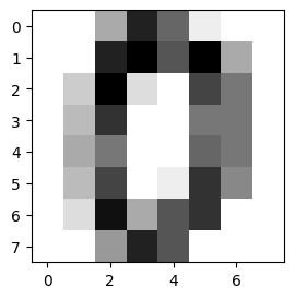
To showcase more advanced queries like conditional sampling and MPE (Most Probable Explanation) we take a look at a dataset with more features. Below, we load the digits dataset. This dataset contains 1797 8x8 images of digits 0 to 9.

[44]:

import matplotlib.pyplot as plt

from sklearn import datasets

# Load the digits dataset
digits = datasets.load_digits()

# Display the last digit
plt.figure(1, figsize=(3, 3))
plt.imshow(digits.images[0], cmap=plt.cm.gray_r, interpolation="nearest")
plt.show()

X = digits.data  # shape (1797, 64)
y = digits.target  # shape (1797,)

X_tensor = torch.tensor(X, dtype=torch.float32)
y_tensor = torch.tensor(y, dtype=torch.long)

dataset = TensorDataset(X_tensor, y_tensor)
dataloader = DataLoader(dataset, batch_size=128, shuffle=True)

print(X_tensor.shape)
print(X_tensor.min(), X_tensor.max())

torch.Size([1797, 64])
tensor(0.) tensor(16.)

Again we create a Rat SPN, but this time we use a Binomial distribution for the leaf layer.

[45]:

from spflow.modules.leaves import Binomial

depth = 3
n_region_nodes = 5
num_leaves = 5
num_repetitions = 2
n_root_nodes = 1
num_feature = 64
n = torch.tensor(16)  # total count for binomial distribution

scope = Scope(list(range(0, num_feature)))

rat_leaf_layer = Binomial(scope=scope, total_count=n, out_channels=num_leaves, num_repetitions=num_repetitions)
rat = RatSPN(
    leaf_modules=[rat_leaf_layer],
    n_root_nodes=n_root_nodes,
    n_region_nodes=n_region_nodes,
    num_repetitions=num_repetitions,
    depth=depth,
    outer_product=True,
    split_mode=SplitMode.consecutive(),
)
print(rat.to_str())

RatSPN [D=1, C=1, R=2] → scope: 0-63
└─ RepetitionMixingLayer [D=1, C=1] [weights: (1, 1, 2)] → scope: 0-63
   └─ Sum [D=1, C=1] [weights: (1, 25, 1, 2)] → scope: 0-63
      └─ OuterProduct [D=1, C=25] → scope: 0-63
         └─ SplitConsecutive [D=2, C=5] → scope: 0-63
            └─ Sum [D=2, C=5] [weights: (2, 25, 5, 2)] → scope: 0-63
               └─ OuterProduct [D=2, C=25] → scope: 0-63
                  └─ SplitConsecutive [D=4, C=5] → scope: 0-63
                     └─ Sum [D=4, C=5] [weights: (4, 25, 5, 2)] → scope: 0-63
                        └─ OuterProduct [D=4, C=25] → scope: 0-63
                           └─ SplitConsecutive [D=8, C=5] → scope: 0-63
                              └─ Factorize [D=8, C=5] → scope: 0-63
                                 └─ Binomial [D=64, C=5] → scope: 0-63

[46]:

train_gradient_descent(rat, dataloader, epochs=20, lr=0.1)

Below is a visualization of some samples drawn from the Spn

[47]:

samples = rat.sample(num_samples=5)
print(samples.shape)

for i in range(5):
    img = samples[i].reshape(8, 8)  # reshape back to 2D
    plt.subplot(1, 5, i + 1)
    plt.imshow(img, cmap="gray")
    plt.axis("off")
plt.show()

torch.Size([5, 64])

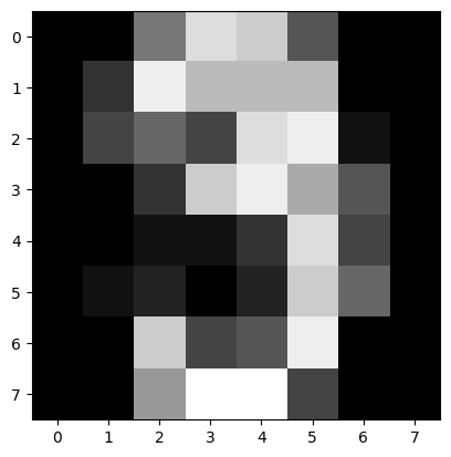
Now can show some more advanced queries. One of them is getting the MPE. It returns the most probable state of the probabilistic circuit. This is often helpful to generate more clear samples and a good indicator whether the model could learn the data or not, which is not always evident with regular samples.

[48]:

mpe = rat.sample(num_samples=1, is_mpe=True)
plt.imshow(mpe.reshape(8, 8), cmap="gray")
plt.show()

And at last we want to sample, given some evidence. In this example, the lower half of the image is given, and we want to sample the upper half given the lower half. This time, instead of explicitly defining a sampling context, we use the sample_with_evidence method. The method allows the user to just input the evidence and let the library internally handle the creation of the sampling context. This becomes handy if you have evidence but not multiple channel to sample from.

[49]:

evidence = X_tensor[0]
evidence[:32] = torch.nan
plt.imshow(evidence.reshape(8, 8), cmap="gray")
plt.show()
evidence = evidence.unsqueeze(0)
print(evidence.shape)
samples = rat.sample_with_evidence(evidence=evidence)
plt.imshow(samples.reshape(8, 8), cmap="gray")
plt.show()

torch.Size([1, 64])

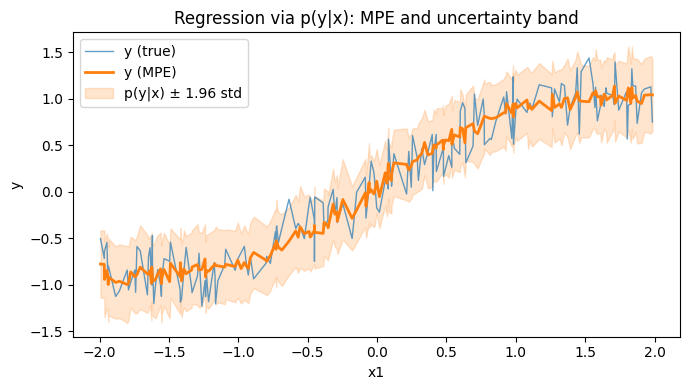
Regression via MPE (continuous target)¶

In SPFlow, you can model regression as a joint density p(y, x) (where y is continuous). After training by maximizing log-likelihood, you can predict with MPE:

Build an evidence tensor where the input features x are set.
Set the target y to NaN.
Call model.mpe(data=evidence) to fill in the most probable y.

Below is a minimal example that learns p(y, x) = p(x) p(y|x) and evaluates prediction quality with MSE.

[64]:

import torch
import torch.nn.functional as F
import matplotlib.pyplot as plt
from torch import nn
from torch.utils.data import DataLoader, TensorDataset

from spflow.learn import train_gradient_descent
from spflow.meta import Scope
from spflow.modules.leaves import Normal
from spflow.modules.products import Product

torch.manual_seed(0)


def make_data(num_samples: int) -> torch.Tensor:
    x = (torch.rand(num_samples, 3) * 4.0) - 2.0
    y = (
        torch.sin(x[:, 0:1])
        + 0.05 * x[:, 1:2].pow(2)
        - 0.025 * x[:, 2:3]
        + 0.20 * torch.randn(num_samples, 1)
    )
    return torch.cat([y, x], dim=1).to(torch.float32)


train_data = make_data(800)  # columns: [y, x1, x2, x3]
test_data = make_data(200)


class ConditionalNormalParams(nn.Module):
    def __init__(self, in_features: int, hidden_features: int = 32) -> None:
        super().__init__()
        self.net = nn.Sequential(
            nn.Linear(in_features, hidden_features),
            nn.Tanh(),
            nn.Linear(hidden_features, 2),
        )

    def forward(self, evidence: torch.Tensor) -> dict[str, torch.Tensor]:
        out = self.net(evidence)
        loc = out[:, 0:1]
        raw_scale = out[:, 1:2]
        scale = F.softplus(raw_scale) + 1e-3
        return {
            "loc": loc.unsqueeze(2).unsqueeze(-1),
            "scale": scale.unsqueeze(2).unsqueeze(-1),
        }


# Joint model p(y, x) = p(x) * p(y|x)
y_given_x = Normal(
    scope=Scope(query=[0], evidence=[1, 2, 3]),
    out_channels=1,
    num_repetitions=1,
    parameter_fn=ConditionalNormalParams(in_features=3),
)
x_marginal = Normal(scope=Scope(query=[1, 2, 3]), out_channels=1, num_repetitions=1)
model = Product(inputs=[y_given_x, x_marginal])


@torch.no_grad()
def predict_y_mpe(model, data: torch.Tensor) -> torch.Tensor:
    evidence = data.clone()
    evidence[:, 0] = torch.nan
    return model.mpe(data=evidence)[:, 0]


@torch.no_grad()
def regression_mse(model, data: torch.Tensor) -> torch.Tensor:
    y_pred = predict_y_mpe(model, data)
    return torch.mean((y_pred - data[:, 0]).pow(2))


print("MSE before:", float(regression_mse(model, test_data)))

loader = DataLoader(TensorDataset(train_data), batch_size=64, shuffle=True)
train_gradient_descent(model, loader, epochs=20, lr=0.05)

print("MSE after:", float(regression_mse(model, test_data)))

# Plot conditional distribution p(y|x) (±1 std) and the MPE prediction, as a function of x1
x1 = test_data[:, 1].detach().cpu()
y_true = test_data[:, 0].detach().cpu()

# Conditional distribution parameters for y|x come from the conditional leaf
x_evidence = test_data[:, [1, 2, 3]]
dist_y_given_x = y_given_x.conditional_distribution(x_evidence)

y_mpe = predict_y_mpe(model, test_data).detach().cpu()
y_std = dist_y_given_x.stddev.detach().cpu().squeeze()

order = torch.argsort(x1)
x1_sorted = x1[order]
y_true_sorted = y_true[order]
y_mpe_sorted = y_mpe[order]
y_std_sorted = y_std[order]

plt.figure(figsize=(7, 4))
plt.plot(x1_sorted, y_true_sorted, linewidth=1.0, alpha=0.7, label="y (true)")
mpe_line = plt.plot(x1_sorted, y_mpe_sorted, linewidth=2.0, label="y (MPE)")[0]
mpe_color = mpe_line.get_color()
plt.fill_between(
    x1_sorted,
    (y_mpe_sorted - 1.96 * y_std_sorted),
    (y_mpe_sorted + 1.96 * y_std_sorted),
    color=mpe_color,
    alpha=0.2,
    label="p(y|x) ± 1.96 std",
)
plt.xlabel("x1")
plt.ylabel("y")
plt.title("Regression via p(y|x): MPE and uncertainty band")
plt.legend()
plt.tight_layout()
plt.show()

MSE before: 0.8204181790351868
MSE after: 0.04302353784441948